Python code: read a price series and describe it (free download)

Python code: read a price series and describe it (free download)
A price series is really just a list of numbers with dates on it: what something cost on each day. Reading one properly, that is, how much it changed, how much it moved around and what shape it has, is the first job for anyone who follows markets, and it is just as useful for a small business owner who wants to compare a product's prices with those of the same months a year earlier. This Python program does exactly that: it opens a file with two columns, works out the summary of the series and draws it on the console with characters, with no chart window and no third-party libraries. It is written for people who do not code: you run it with one command and there is nothing else to install.
⬇ Download the code (ZIP)Notice: this program is educational material. This is not a recommendation to buy or to sell. The sample prices that travel inside the ZIP are made up and the historical data is quoted only for practice. A past result guarantees nothing about the future. Ask an authorised professional before investing.
What the ZIP brings
| File | What it is |
|---|---|
| serie_precios.py | The whole program, commented in English. It uses the Python standard library only. |
| datos/prices.csv | The made-up sample series: 180 daily closes, with the columns date and close. |
| datos/real_prices.csv | Two historical series quoted only for practice: bitcoin in dollars and the S&P 500 index, one row per asset. |
| salida_ejemplo.txt | The full output of the program, copied as it is, chart included. |
| README.md | The instructions and the written legal notice. |
Where the historical data comes from: CoinGecko (api.coingecko.com) for bitcoin and the Federal Reserve Bank of St. Louis, SP500 series, for the index (https://fred.stlouisfed.org/series/SP500). Both series were downloaded on 25 September 2026 and are used as practice data only. If you would rather work with your own numbers, replace the file in the datos/ folder with your own CSV: the format is explained in the table below and you do not have to touch a single line of the program.
What the program does
- Reads datos/prices.csv, the made-up sample series, with 180 daily closes.
- Works out the daily return of every day: how much the close moved from the day before, in percent.
- Summarises the series: number of rows, first and last date, minimum and maximum close, first and last close, total change, average daily change and volatility.
- Checks its own arithmetic: that the last close is the one in the last row of the file and that the total change, computed in two different ways, comes out the same.
- Repeats the same summary for datos/real_prices.csv, this time grouping by asset: one row per asset.
- Draws the sample series on the console as sixty columns of block characters, with a legend pointing at the minimum and the maximum.
- Saves the whole summary to salida/resumen_series.csv, ready to open in Excel.
- Prints the legal notice at the start and at the end.
How to run it
You need Python 3.11 or newer. On Windows you install it from python.org and it is worth ticking the box that adds Python to the PATH. Then unzip the package into any folder, open a terminal in that folder and type the command below. A quick way to get there is to right-click the folder and pick the option that opens a terminal right in it.
python serie_precios.py
There is nothing else to install: the program uses the standard library only. It does not need an internet connection either, because both price files travel inside the ZIP. If the Windows console cannot draw the block characters of the chart, the program itself switches its output to UTF-8 instead of crashing, so it runs the same on Windows, on Linux and on a Mac.
The format of the data file
| Column | What it holds | Example |
|---|---|---|
| date | The day, as year-month-day | 2026-01-02 |
| close | The closing price of that day, with decimals | 99.94 |
The file with the real series adds one more column, asset, holding the name of the asset so the program knows where one series starts and the next one begins. The headers go on the first line and every row is one day. If your file holds more than a hundred days, so much the better: the volatility and the chart read more calmly. The only things to respect are the order of the columns and the decimal point inside the file; the program takes care of the rest.
The code, explained
The program is under two hundred and fifty lines long and it is commented in English. These are the five pieces worth understanding, copied word for word from the file inside the ZIP.
The tools and the paths
Those four imports are the whole toolbox: csv to read the file, sys to find out how the console draws, Decimal so that prices and percentages do not drag rounding errors along, and pathlib to build paths that work the same on Windows, Linux and Mac. The BASE variable is the folder of the program itself, which is why the program runs from anywhere: it does not depend on where you happen to be standing when you call it.
import csv                                        # csv: read the price file without installing anything
import sys                                        # sys: find out which character set the console draws with
from decimal import Decimal, ROUND_HALF_UP        # Decimal: exact prices and percentages, no binary surprises
from pathlib import Path                          # pathlib: paths that work on Windows, Linux and Mac

# Folder of this very file: the program runs from anywhere
BASE = Path(__file__).resolve().parent
ENTRADA = BASE / "datos" / "prices.csv"      # made-up sample series, shipped inside the ZIP
ENTRADA_REAL = BASE / "datos" / "real_prices.csv"    # historical series quoted only for practice (two assets)
SALIDA = BASE / "salida" / "resumen_series.csv"   # summary of the series, ready to open in Excel
The daily return: the raw material
The return of a day is how much the close moved compared with the day before, in percent. The function walks through the closes with an index and divides each one by the previous one; the minus one leaves the change as a clean percentage. With that list in hand you can measure the average change and, above all, the volatility. The function hands back a dictionary with the dates, the extremes, the first close, the last close and the three percentages of the summary.
def estadisticas(filas: list[dict]) -> dict:
    """Computes the summary of the series: dates, extremes, change and volatility."""
    fechas = [fila["date"] for fila in filas]
    cierres = [Decimal(fila["close"]) for fila in filas]
    # Daily return (%): how much the close moved from one day to the next
    retornos = [(cierres[i] / cierres[i - 1] - 1) * CIEN for i in range(1, len(cierres))]
Volatility: a standard deviation
Volatility is nothing more than the standard deviation of those returns: a single number that sums up how far the daily changes sit from their average. If the price moves little, the deviation is small; if it jumps around, it grows. The population formula is used, dividing by the number of returns and not by one less than that number, and the square root of the result is the figure you see. Comparing this number between two series says far more than staring at the closes on their own.
def desviacion(valores: list[Decimal]) -> Decimal:
    """Population standard deviation of a list of numbers."""
    media = sum(valores) / len(valores)
    # Population formula: the variance divides by the number of returns, not by n-1
    varianza = sum((valor - media) ** 2 for valor in valores) / len(valores)
    return varianza.sqrt()
The console chart: one level per character
A terminal has no windows, so the chart is drawn with characters. The function nivel maps a close to a number from zero to seven, which is the position of the character inside the ladder of blocks; the value is scaled between the minimum and the maximum of the series. Then the dibujar function averages several days into each of the sixty columns and prints the line. That is how you see the shape of the series at a glance, without opening a spreadsheet.
def nivel(valor: Decimal, minimo: Decimal, maximo: Decimal) -> int:
    """Maps a close to a level from 0 to 7: the index of the chart character."""
    if maximo == minimo:
        return 0
    posicion = (valor - minimo) / (maximo - minimo)
    indice = (posicion * (len(ESCALONES) - 1)).quantize(Decimal("1"), rounding=ROUND_HALF_UP)
    return max(0, min(len(ESCALONES) - 1, int(indice)))
The checks: do not trust yourself
The program works out the last close in two ways and the total change in two ways, and then compares them. When both sums agree it prints that they tie. It is a healthy habit: when a number comes out the same along two different roads, you trust it far more than a lone result. In practice, that is what separates a summary you can use from a figure somebody made up.
def comprobar(filas: list[dict], datos: dict) -> None:
    """Prints the two checks of the series."""
    # Check 1: the last close is the close of the last row of the file
    cuadra1 = Decimal(filas[-1]["close"]) == datos["ultimo"]
    # Check 2: the total change, computed another way, must give the same figure
    directa = (datos["ultimo"] / datos["primero"] - 1) * CIEN
    cuadra2 = redondear(directa * 10000) == redondear(datos["var_total"] * 10000)
What you will see on the screen
When you run it, the first thing on the screen is the legal notice; then comes the table for the sample series with its summary: 180 rows, the first and the last date of the file and the three figures that always turn up. The two checks follow underneath. For the real series, the table prints one row per asset. This is a piece of the real output, copied as it is:
SAMPLE SERIES
---------------------------------------------------------------------------------------------------------------------------------------------------
Series                   Items        Start         End      Minimum      Maximum        First         Last    Change % Avg. daily %   Volatility %
---------------------------------------------------------------------------------------------------------------------------------------------------
Sample                   180     2026-01-02  2026-06-30        92.25       123.61        99.94       117.24     17.31 %       0.10 %         1.23 %
---------------------------------------------------------------------------------------------------------------------------------------------------
    Check: last close = last row of the file: TIES
    Check: total change = (last/first - 1) × 100: TIES
REAL DATA
  Source of the real data: CoinGecko, api.coingecko.com and Federal Reserve Bank of St. Louis (SP500 series), downloaded on 2026-09-25
SUMMARY BY ASSET
---------------------------------------------------------------------------------------------------------------------------------------------------
Series                   Items        Start         End      Minimum      Maximum        First         Last    Change % Avg. daily %   Volatility %
---------------------------------------------------------------------------------------------------------------------------------------------------
Bitcoin (USD)            120     2026-05-30  2026-09-25    58,566.09    86,596.74    73,500.92    83,706.64     13.89 %       0.13 %         2.16 %
S&P 500 (index)          120     2026-04-06  2026-09-24     6,611.83     7,798.99     6,611.83     7,704.13     16.52 %       0.13 %         0.79 %
---------------------------------------------------------------------------------------------------------------------------------------------------
And at the end comes the teaching moment: the chart. Every character is the average of three consecutive days, and the ladder of blocks runs from the lowest level to the highest. Read from left to right it shows the shape of those months: up, a pause, a flat stretch and up again, with the lowest point marked around the middle of the period. A chart made of characters predicts nothing, but it orders the eye far better than a plain list of numbers.
CHART OF THE SAMPLE SERIES (60 columns)
---------------------------------------------------------------------------------------------------------------------------------------------------
  ▃▃▃▄▄▄▃▃▄▄▄▅▅▅▅▅▅▅▅▆▅▄▄▃▃▂▂▂▂▂▂▁▁▁▂▂▃▃▃▃▃▄▄▅▆▆▇▇▇▇▇█▇▇▇▇▇▇▆▇
---------------------------------------------------------------------------------------------------------------------------------------------------
Legend: ▁ minimum 92.25 (2026-04-08) | █ maximum 123.61 (2026-06-04)
Common mistakes and tips
- If the terminal answers that python is not a recognised program, try the name python3, which is what Linux and some Macs use.
- Run the program from the folder where you unzipped it, or hand it the full path of the file. If you move it somewhere else, the datos/ folder has to travel with it.
- If you change the price file, keep the headers and the column names as they are. One extra comma in a row muddles the whole analysis without a single warning.
- Mind the decimal point in the data file: the program reads a point, not a comma, even though it prints the numbers in the local format afterwards.
- A series of only a few days gives a volatility you cannot rely on. Below twenty closes the summary is practice, not a basis for conclusions.
- If a day is missing from the file, the jump counts as a single return. Gaps do not fill themselves in.
When this is not enough
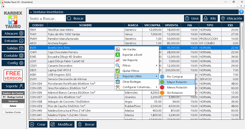
This program is a good exercise and it handles a series, or two. Once a small business's inventory enters the picture, things change: purchases, sales, balances per warehouse, costs and the trail you need to leave behind so a movement can be reviewed months later. That is where Kardex Tauro starts to make sense, because it keeps the inventory and the real cost and keeps the history. If your problem is one price file, stay with the script; when the movements multiply and the figures have to tie in with accounting, the script falls short.
Notice: this article and the program are educational material. This is not a recommendation to buy or to sell. The source of the data is cited above and the ZIP carries the written legal notice together with the instructions. The sample prices are made up and the historical ones are quoted only for practice: a past result guarantees nothing about the future, so ask an authorised professional before investing.
⬇ Download the code (ZIP)Download the ZIP, run the program with a single command line and watch your first price series described with numbers and with characters. Then swap the file for your own prices and compare: the same exercise, with data that matters to you.